Artificial Intelligence Nanodegree
Convolutional Neural Networks
Project: Write an Algorithm for a Dog Identification App
In this notebook, some template code has already been provided for you, and you will need to implement additional functionality to successfully complete this project. You will not need to modify the included code beyond what is requested. Sections that begin with '(IMPLEMENTATION)' in the header indicate that the following block of code will require additional functionality which you must provide. Instructions will be provided for each section, and the specifics of the implementation are marked in the code block with a 'TODO' statement. Please be sure to read the instructions carefully!
Note: Once you have completed all of the code implementations, you need to finalize your work by exporting the iPython Notebook as an HTML document. Before exporting the notebook to html, all of the code cells need to have been run so that reviewers can see the final implementation and output. You can then export the notebook by using the menu above and navigating to \n", "File -> Download as -> HTML (.html). Include the finished document along with this notebook as your submission.
In addition to implementing code, there will be questions that you must answer which relate to the project and your implementation. Each section where you will answer a question is preceded by a 'Question X' header. Carefully read each question and provide thorough answers in the following text boxes that begin with 'Answer:'. Your project submission will be evaluated based on your answers to each of the questions and the implementation you provide.
Note: Code and Markdown cells can be executed using the Shift + Enter keyboard shortcut. Markdown cells can be edited by double-clicking the cell to enter edit mode.
The rubric contains optional "Stand Out Suggestions" for enhancing the project beyond the minimum requirements. If you decide to pursue the "Stand Out Suggestions", you should include the code in this IPython notebook.
Why We're Here
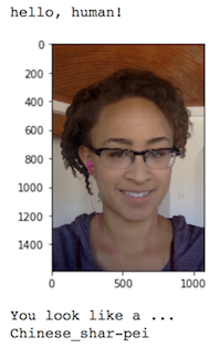
In this notebook, you will make the first steps towards developing an algorithm that could be used as part of a mobile or web app. At the end of this project, your code will accept any user-supplied image as input. If a dog is detected in the image, it will provide an estimate of the dog's breed. If a human is detected, it will provide an estimate of the dog breed that is most resembling. The image below displays potential sample output of your finished project (... but we expect that each student's algorithm will behave differently!).
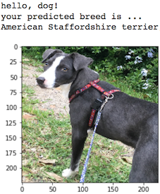
In this real-world setting, you will need to piece together a series of models to perform different tasks; for instance, the algorithm that detects humans in an image will be different from the CNN that infers dog breed. There are many points of possible failure, and no perfect algorithm exists. Your imperfect solution will nonetheless create a fun user experience!
The Road Ahead
We break the notebook into separate steps. Feel free to use the links below to navigate the notebook.
- Step 0: Import Datasets
- Step 1: Detect Humans
- Step 2: Detect Dogs
- Step 3: Create a CNN to Classify Dog Breeds (from Scratch)
- Step 4: Use a CNN to Classify Dog Breeds (using Transfer Learning)
- Step 5: Create a CNN to Classify Dog Breeds (using Transfer Learning)
- Step 6: Write your Algorithm
- Step 7: Test Your Algorithm
Step 0: Import Datasets
Import Dog Dataset
In the code cell below, we import a dataset of dog images. We populate a few variables through the use of the load_files function from the scikit-learn library:
train_files,valid_files,test_files- numpy arrays containing file paths to imagestrain_targets,valid_targets,test_targets- numpy arrays containing onehot-encoded classification labelsdog_names- list of string-valued dog breed names for translating labels
from sklearn.datasets import load_files
from keras.utils import np_utils
import numpy as np
from glob import glob

# define function to load train, test, and validation datasets
def load_dataset(path):
    data = load_files(path)
    dog_files = np.array(data['filenames'])
    dog_targets = np_utils.to_categorical(np.array(data['target']), 133)
    return dog_files, dog_targets

# load train, test, and validation datasets
train_files, train_targets = load_dataset('dogImages/train')
valid_files, valid_targets = load_dataset('dogImages/valid')
test_files, test_targets = load_dataset('dogImages/test')

# load list of dog names
dog_names = [item[20:-1] for item in sorted(glob("dogImages/train/*/"))]

# print statistics about the dataset
print('There are %d total dog categories.' % len(dog_names))
print('There are %s total dog images.\n' % len(np.hstack([train_files, valid_files, test_files])))
print('There are %d training dog images.' % len(train_files))
print('There are %d validation dog images.' % len(valid_files))
print('There are %d test dog images.'% len(test_files))
Import Human Dataset
In the code cell below, we import a dataset of human images, where the file paths are stored in the numpy array human_files.
import random
# changed these lines, so that I can later use the random seed again
RS = 8675309
random.seed(RS)

# load filenames in shuffled human dataset
human_files = np.array(glob("lfw/*/*"))
random.shuffle(human_files)

# print statistics about the dataset
print('There are %d total human images.' % len(human_files))
Step 1: Detect Humans
We use OpenCV's implementation of Haar feature-based cascade classifiers to detect human faces in images. OpenCV provides many pre-trained face detectors, stored as XML files on github. We have downloaded one of these detectors and stored it in the haarcascades directory.
In the next code cell, we demonstrate how to use this detector to find human faces in a sample image.
import cv2
import matplotlib.pyplot as plt
%matplotlib inline

# extract pre-trained face detector
face_cascade = cv2.CascadeClassifier('haarcascades/haarcascade_frontalface_alt.xml')

# load color (BGR) image
img = cv2.imread(human_files[3])
# convert BGR image to grayscale
gray = cv2.cvtColor(img, cv2.COLOR_BGR2GRAY)

# find faces in image
faces = face_cascade.detectMultiScale(gray)

# print number of faces detected in the image
print('Number of faces detected:', len(faces))

# get bounding box for each detected face
for (x,y,w,h) in faces:
    # add bounding box to color image
    cv2.rectangle(img,(x,y),(x+w,y+h),(255,0,0),2)

# convert BGR image to RGB for plotting
cv_rgb = cv2.cvtColor(img, cv2.COLOR_BGR2RGB)

# display the image, along with bounding box
plt.imshow(cv_rgb)
plt.show()

Before using any of the face detectors, it is standard procedure to convert the images to grayscale. The detectMultiScale function executes the classifier stored in face_cascade and takes the grayscale image as a parameter.
In the above code, faces is a numpy array of detected faces, where each row corresponds to a detected face. Each detected face is a 1D array with four entries that specifies the bounding box of the detected face. The first two entries in the array (extracted in the above code as x and y) specify the horizontal and vertical positions of the top left corner of the bounding box. The last two entries in the array (extracted here as w and h) specify the width and height of the box.
Write a Human Face Detector
We can use this procedure to write a function that returns True if a human face is detected in an image and False otherwise. This function, aptly named face_detector, takes a string-valued file path to an image as input and appears in the code block below.
# returns "True" if face is detected in image stored at img_path
def face_detector(img_path):
    img = cv2.imread(img_path)
    gray = cv2.cvtColor(img, cv2.COLOR_BGR2GRAY)
    faces = face_cascade.detectMultiScale(gray)
    return len(faces) > 0
(IMPLEMENTATION) Assess the Human Face Detector
Question 1: Use the code cell below to test the performance of the face_detector function.
- What percentage of the first 100 images in
human_fileshave a detected human face? - What percentage of the first 100 images in
dog_fileshave a detected human face?
Ideally, we would like 100% of human images with a detected face and 0% of dog images with a detected face. You will see that our algorithm falls short of this goal, but still gives acceptable performance. We extract the file paths for the first 100 images from each of the datasets and store them in the numpy arrays human_files_short and dog_files_short.
Answer:
human_files_short = human_files[:100]
dog_files_short = train_files[:100]
# Do NOT modify the code above this line.

## TODO: Test the performance of the face_detector algorithm
## on the images in human_files_short and dog_files_short.
Helper Functions
I am writing some helper functions for this task, since I will use them again later.
from mpl_toolkits.axes_grid1 import ImageGrid
from keras.preprocessing import image as keras_image_preprocess

## My functions are very general, since I want to reuse them later on

# Some helper functions
# ------------------------------------------------------------------------

# returns the image as a numpy array
def read_img(filepath, size):
    img = keras_image_preprocess.load_img(filepath, target_size=size)
    array = keras_image_preprocess.img_to_array(img)
    return array

# shows images from list both as filepathes and as images in a grid
def show_image_grid(img_pathes):
    image_count = len(img_pathes)
    cols = min(image_count, 4) # nr of images in one row
    rows = (image_count // 4) + 1 # nr of rows
    fig_width = cols * 2
    fig_height = rows * 2
    fig = plt.figure(1, (fig_width, fig_height))
    grid = ImageGrid(fig, 111, # similar to subplot(111)
                    nrows_ncols = (rows, cols), # creates grid
                    axes_pad=0.1, # pad between axes in inch.
                    )

    for i in range(image_count):
        im = read_img(img_pathes[i], (224, 224))
        grid[i].imshow(im / 255.) # show image in grid element
    plt.show()


# Determines the accuracy on a list of images given by their pathes:
# ------------------------------------------------------------------------
# Parameters:
# - title: the title to print out
# - img_path_list: a list of image file pathes
# - detector: a detector function, that takes the image path and returns a predicted value
# - groundtruth: List of groundtruth values for the image paths
# - show_fails: show incorrectly classified images in a grid
# Result:
# - has no output, but prints the accuracy and the images, that have been misclassified in a grid
def get_detector_accurancy(title, img_path_list, detector, ground_truth, show_fails=True):
    """the detector accuracy is determined, also the images that have been incorrectly classified
    are remebered"""
    detected = np.array([detector(img_path) for img_path in img_path_list])
    ground_truth = np.array(ground_truth)
    accuracy = 100*np.sum(detected==ground_truth)/len(detected)
    incorrect = img_path_list[np.where(detected!=ground_truth)]
    print("{} were classified with an accuracy of {} %\n".format(title, accuracy))

    # show incorrectly classified images in a grid
    if show_fails and len(incorrect) > 0:
        print("Incorrectly classified:", incorrect)
        show_image_grid(incorrect)
get_detector_accurancy(title="Humans",
                       img_path_list=human_files_short,
                       detector=face_detector,
                       ground_truth=[True for img_path in human_files_short])

get_detector_accurancy(title="Dogs",
                       img_path_list=dog_files_short,
                       detector=face_detector,
                       ground_truth=[False for img_path in dog_files_short])

Answer to Question1
What percentage of the first 100 images in human_files have a detected human face?
98 % of the first 100 images in human_files had a human face detected.
What percentage of the first 100 images in dog_files have a detected human face?
11.0 % of the first 100 images in dog_files had a human face detected.
Question 2: This algorithmic choice necessitates that we communicate to the user that we accept human images only when they provide a clear view of a face (otherwise, we risk having unneccessarily frustrated users!). In your opinion, is this a reasonable expectation to pose on the user? If not, can you think of a way to detect humans in images that does not necessitate an image with a clearly presented face?
Answer:
We suggest the face detector from OpenCV as a potential way to detect human images in your algorithm, but you are free to explore other approaches, especially approaches that make use of deep learning :). Please use the code cell below to design and test your own face detection algorithm. If you decide to pursue this optional task, report performance on each of the datasets.
## (Optional) TODO: Report the performance of another
## face detection algorithm on the LFW dataset
### Feel free to use as many code cells as needed.
Answer to Question2: Assess human face detector
Flaws of the face detector
The Human Face detecto:
- does not detect faces, that do not show a frontal face.
- it detects the faces for dogs as well
Are Haar cascades for face detection are an appropriate technique for human detection?
- No, I don't think they are. The can point to were they suspect a face, but I think the measurements are not flexible enough to pick up on different head positions. Also they might take animal heads for humans if the proportions are similar. This seems to be the case for dogs.
My own your own face detection algorithm
Transfer Learning for Human Dog Detection
I decided to try Transfer Learning for Human Detection
Data
I just used the data, that was already there: human_files for humans and dog_files for dogs
Features
My idea was to explore the bottleneck features od ResNet50 for this task. For the dogs the bottleneck feature were already given. I just had to produce them for the humans.
TSNE
I usually try to visualize how good the features are for the task at hand by looking at a TSNE projection whenever that is possible.
Categorical Crossentropy
I was aiming for Categorical Entrophy rather then Binary Classification since I was hoping to detect, that an image was neither human nor a dog would be detectable by the propabilities for both classes being undecisive. That hpe turned out to be false though.
Human Dog Detector
It turned out that my detector has a bias towards dogs: everything not human was classified as dog. That made it actually useful in detecting humans.
Implementation
You find my Implementation in the cells below. Whenever possible I try locally to get the data from files, in order to make the notebook faster to run through. It is not possible to store the file on github though.
Run Options
Since computing the HumanDetector is time expensive, I stored the results in files and give the option to recompute them with the variable RECOMPUTE_HUMAN_DOG_DETECTOR_MODEL, which is preset to False, but can be changed to True.
My Human Dog Detector
Human Dog Detector Step 1:
- Loading the human images from human_files
- stacking the dog_images all to one dog_file
Only recomputed on request
- the computation of my model was time intense, therefore it is only recomputed on request: if you set
RECOMPUTE_HUMAN_DOG_DETECTOR_MODELtoTrue. I initially thought of storing the intermediated tensors, but this hit a storage limit in github. Therefore I chose this solution.
RECOMPUTE_HUMAN_DOG_DETECTOR_MODEL = False
# define function to load train, test, and validation datasets
def load_dataset(path):
    data = load_files(path)
    human_files = np.array(data['filenames'])
    return human_files

if RECOMPUTE_HUMAN_DOG_DETECTOR_MODEL:
    # load train, test, and validation datasets
    human_files = load_dataset('lfw')
    dog_files = np.hstack([train_files, valid_files, test_files])

    # print statistics about the dataset
    print('There are %s total human images.\n' % len(np.hstack([human_files])))
    print('There are %s total dog images.\n' % len(np.hstack([dog_files])))
Human Dog Detector Step 2: getting bottleneck features for the human_images
- this is also needed for the prediction later on, so also in the case that the model is not recomputed.
from keras.applications.resnet50 import preprocess_input as resnet50_preprocess_input
from keras.applications.resnet50 import ResNet50
from keras.preprocessing import image

# the model is only defined once with top of since we want the features just before the imagenet classes are received.
model_resnet50 = ResNet50(include_top=False, weights='imagenet')

# computing the features by making a forward pass through resnet50 from keras
def get_resnet50_features(img_path):
    img = image.load_img(img_path, target_size=(224, 224))
    # convert PIL.Image.Image type to 3D tensor with shape (224, 224, 3)
    x = image.img_to_array(img)
    # convert 3D tensor to 4D tensor with shape (1, 224, 224, 3) and return 4D tensor
    x = np.expand_dims(x, axis=0)
    # get the feature by a forward pass through the model
    features = model_resnet50.predict(resnet50_preprocess_input(x))
    return features
Compute the human tensors
- locally I stored them to a file, so that I had to compute them ony once. But the file turned out to be to big for Github.
if RECOMPUTE_HUMAN_DOG_DETECTOR_MODEL:
# since this computationaly expensive I try to get the tensors from file if possible
    try:
        human_tensors = np.load('myfiles/HumanDogDetector/human_resnet50_tensors.npy')
    except FileNotFoundError:
        # initialize array
        human_tensors = np.zeros((human_files.shape[0], 2048))
        # compute features from pretrained resnet50
        for i in tqdm(range(human_tensors.shape[0])):
            human_tensors[i] = get_resnet50_features(human_files[i])
        # saving the bottleneckfeatures for later
        np.save('myfiles/HumanDogDetector/human_resnet50_tensors', human_tensors)
        print("Computed {} human tensors of shape {} and saved them to a file.".format(
            len(human_tensors), human_tensors.shape))
    else:
        print("Loaded {} human tensors of shape {} from file".format(len(human_tensors), human_tensors.shape))
Human Dog Detector Step 3: getting bottleneck features for the dog_images
These features have been given to us, so that I can just load them from the given files
- I stack test, train and validation data all together, since I have to shuffle and split the data again later anyway.
### Obtain bottleneck features from ResNet50 and squeeze them
if RECOMPUTE_HUMAN_DOG_DETECTOR_MODEL:
    bottleneck_features = np.load('bottleneck_features/DogResnet50Data.npz')
    dog_tensors = np.vstack([bottleneck_features['train'], bottleneck_features['valid'], bottleneck_features['test']])
    dog_tensors = np.squeeze(dog_tensors)
    print("There are {} dog tensors of shape {}".format(len(dog_tensors), dog_tensors.shape))
Human Detector Step 4: Mixing the datasets and targets
- stacking everything together: tensors and targets
- one hot encoding of both classes humans and dogs
if RECOMPUTE_HUMAN_DOG_DETECTOR_MODEL:
    ### Obtain bottleneck features from ResNet50 and squeeze them
    nr_classes = 2

    # one hot encoding humen classes
    human_targets = np.hstack([np.zeros((human_tensors.shape[0],1)), np.ones((human_tensors.shape[0],1))])
    print("Human targets are now of shape", human_targets.shape)
    print("Human targets look like", human_targets[0])

    # one hot encoding dog classes
    dog_targets = np.hstack([np.ones((dog_tensors.shape[0],1)), np.zeros((dog_tensors.shape[0],1))])
    print("Dog targets are now of shape", dog_targets.shape)
    print("Dog targets look like", dog_targets[0])

    # stacking tensors and targets together
    dh_tensors = np.vstack([dog_tensors, human_tensors])
    dh_targets = np.vstack([dog_targets, human_targets])
    print("Tensors have now shape", dh_tensors.shape)
    print("Targets have now shape", dh_targets.shape)
else:
    print("""if run with RECOMPUTE_HUMAN_DOG_DETECTOR_MODEL, this cell produces the following output:
    Human targets are now of shape (13233, 2)
    Human targets look like [ 0.  1.]
    Dog targets are now of shape (8351, 2)
    Dog targets look like [ 1.  0.]
    Tensors have now shape (21584, 2048)
    Targets have now shape (21584, 2)""")
Human Dog Detector Step 5: Mixing the datasets and targets
- shuffling the features and targets so that the humans and dogs get mixed
if RECOMPUTE_HUMAN_DOG_DETECTOR_MODEL:
    # shuffle the datasets with Shuffle Split
    from sklearn.model_selection import ShuffleSplit

    splitter_train = ShuffleSplit(n_splits=1, test_size=0.2, random_state=0)
    splitter_train.get_n_splits(dh_tensors, dh_targets)

    # get split indexes
    dh_train_index, dh_test_index = next(splitter_train.split(dh_tensors, dh_targets))
    val_split = int(len(dh_test_index) / 2)
    dh_val_index = dh_test_index[:val_split]
    dh_test_index = dh_test_index[val_split:]

    x_dh_train, y_dh_train = dh_tensors[dh_train_index], dh_targets[dh_train_index]
    x_dh_test, y_dh_test = dh_tensors[dh_test_index], dh_targets[dh_test_index]
    x_dh_val, y_dh_val = dh_tensors[dh_val_index], dh_targets[dh_val_index]

    print("The shapes of train, validation and test tensors and targets are now:\nTensors: {}, {}, {}\nTargets: {}, {}, {}"
          .format(x_dh_train.shape, x_dh_val.shape, x_dh_test.shape, y_dh_train.shape, y_dh_val.shape, y_dh_test.shape))
else:
    print("""if run with RECOMPUTE_HUMAN_DOG_DETECTOR_MODEL, this cell produces the following output:
    The shapes of train, validation and test tensors and targets are now:
    Tensors: (17267, 2048), (2158, 2048), (2159, 2048)
    Targets: (17267, 2), (2158, 2), (2159, 2)""")
Human Dog Detector Step 6: Visualizing the features with TSNE
- can the features set dogs and humans apart?
- do they look promising? I am using the Validation set for this, just because it is smaller then the training dataset and I am just interested in a visualization of the features on a mixed dataset.
# applying TSNE algorithm
from sklearn.manifold import TSNE

def perform_tsne(X):
    proj = TSNE(random_state=RS, verbose=1).fit_transform(X)
    return proj
if RECOMPUTE_HUMAN_DOG_DETECTOR_MODEL:
    # preforming TSNE: this just projects distances of features, so the targets are not necessary
    filepath = 'myfiles/tsnedata/HumanDogResNet50TSNEData'
    try:
        proj_val = np.load(filepath + '.npy')
    except FileNotFoundError:
        proj_val = perform_tsne(x_dh_val)
        np.save(filepath, proj_val)
        print('TSNE projection computed and saved to file.')
    else:
        print('TSNE projection loaded from file.')
else:
    print("""if run with RECOMPUTE_HUMAN_DOG_DETECTOR_MODEL, this cell produces the following output:
    TSNE projection loaded.""")
Helper functions
The plotting of the TSNE map is very general, since I will use it again later for the dog breeds.
- I am getting the palette from file in case seaborn is not installed
# getting the palette for the colors from either seaborn or from file
try:
    import seaborn as sns
    palette = np.array(sns.color_palette("hls", 25))
    np.random.shuffle(palette)
    np.save('myfiles/palette/palette', palette)
except ImportError:
    palette = np.load('myfiles/palette/palette.npy')
# helper function for the tsne plot
import matplotlib.patches as mpatches

# scatter plotting the tsne data
# parameters:
# - x: the data is supposed to be 2 dimensional
# - colors: the target as color codes, the codes should be a range(n) for any integer n < 25: 0,1,2,3,..
# - title: the title of the plot
# - other_color: is there an 'other' class that should be kept in light grey?
# - filename: filename to store the plot
# Output:
# - the plot is displayed and gets saved to file
def scatter(x, colors, legend, title, file_path, other_color=None):
    """this function plots the result
    - x is a two dimensional vector
    - colors is a code that tells how to color them: it corresponds to the target
    - legend is a dictionary that tells what color means what label
    """
    # We choose a color palette with seaborn.
    class_count = len(legend)
    palette_length = class_count
    if other_color:
        palette_length -= 1

    # seaborn
    try:
        palette = np.array(sns.color_palette("hls", palette_length))
    except:
        palette = np.load('myfiles/palette/palette.npy')

    palette = palette[:palette_length]
    if other_color:
        other_color = np.array([0.9, 0.9, 0.9])
        palette = np.vstack([palette, other_color])

    # We create a scatter plot.
    f = plt.figure(figsize=(10, 8))
    ax = plt.subplot(aspect='equal')
    sc = ax.scatter(x[:,0], x[:,1], lw=0, s=40, c=palette[colors.astype(np.int)])

    ax.axis('off') # the axis will not be shown
    ax.axis('tight') # makes sure all data is shown

    # set title
    plt.title(title, fontsize=25)


    # legend with color patches
    patches = []
    for i in range(class_count):
       patch = mpatches.Patch(color=palette[i], label=legend[i])
       patches.append(patch)
    plt.legend(handles=patches, fontsize=10, loc=4)
    plt.savefig(file_path)
# helper function to display and image that is stored in a file
from IPython.display import Image, display
import matplotlib.image as mpimg

# just fetch an image form file and show it
def show_image(img_path):
    img = mpimg.imread(img_path)
    imgplot = plt.imshow(img)

# show image in the original size
def show_image_original(img_path):
    display(Image(img_path))
# plot TSNE projection
file_path = 'myfiles/tsneplots/HumanDogResNet50TSNE.png'
if RECOMPUTE_HUMAN_DOG_DETECTOR_MODEL:
    # Now we call the scatter plot function on our data
    legend = {0:'Dogs', 1: 'Humans'}
    colors = y_dh_val[:, 1]
    scatter(proj_val, colors, legend, title="Resnet Transfer Learning: Humans Dogs", file_path=file_path)
else:
    show_image_original(file_path)

Human Detector Step 7: Build Transfer Learning Model
The TSNE looks promising. Therefore I just put a simple dense layer on top of the features and use categorical_crossentropy as the loss function.
from keras.layers import Dense
from keras.models import Sequential
HUMAN_DOG_DETECTOR_MODEL_INPUT_SHAPE = (2048,)
if RECOMPUTE_HUMAN_DOG_DETECTOR_MODEL:
    assert x_dh_train.shape[1:] == HUMAN_DOG_DETECTOR_MODEL_INPUT_SHAPE
HumanDogDetector_model = Sequential()
HumanDogDetector_model.add(Dense(2, input_shape=HUMAN_DOG_DETECTOR_MODEL_INPUT_SHAPE, activation='softmax'))
HumanDogDetector_model.summary()
if RECOMPUTE_HUMAN_DOG_DETECTOR_MODEL:
    ### Compile the model.
    HumanDogDetector_model.compile(loss='categorical_crossentropy', optimizer='adam', metrics=['accuracy'])
if RECOMPUTE_HUMAN_DOG_DETECTOR_MODEL:
    ### Train the model.
    from keras.callbacks import ModelCheckpoint

    checkpointer = ModelCheckpoint(filepath='saved_models/weights.best.HumanDogDetector.hdf5',
                                   verbose=1, save_best_only=True)

    HumanDogDetector_model.fit(x_dh_train, y_dh_train,
              validation_data=(x_dh_val, y_dh_val),
              epochs=10, batch_size=20, callbacks=[checkpointer], verbose=1)
else:
    print("""if run with RECOMPUTE_HUMAN_DOG_DETECTOR_MODEL, this cell produces the following output:
Train on 17267 samples, validate on 2158 samples
Epoch 1/10
17040/17267 [============================>.] - ETA: 0s - loss: 0.0057 - acc: 0.9983Epoch 00000: val_loss improved from inf to 0.00020, saving model to saved_models/weights.best.HumanDogDetector.hdf5
17267/17267 [==============================] - 2s - loss: 0.0057 - acc: 0.9983 - val_loss: 1.9944e-04 - val_acc: 1.0000
Epoch 2/10
17020/17267 [============================>.] - ETA: 0s - loss: 1.3794e-04 - acc: 1.0000Epoch 00001: val_loss improved from 0.00020 to 0.00007, saving model to saved_models/weights.best.HumanDogDetector.hdf5
17267/17267 [==============================] - 2s - loss: 1.3654e-04 - acc: 1.0000 - val_loss: 7.4057e-05 - val_acc: 1.0000
Epoch 3/10
17100/17267 [============================>.] - ETA: 0s - loss: 5.7718e-05 - acc: 1.0000Epoch 00002: val_loss improved from 0.00007 to 0.00004, saving model to saved_models/weights.best.HumanDogDetector.hdf5
17267/17267 [==============================] - 2s - loss: 5.7736e-05 - acc: 1.0000 - val_loss: 3.8203e-05 - val_acc: 1.0000
Epoch 4/10
17160/17267 [============================>.] - ETA: 0s - loss: 3.1119e-05 - acc: 1.0000Epoch 00003: val_loss improved from 0.00004 to 0.00002, saving model to saved_models/weights.best.HumanDogDetector.hdf5
17267/17267 [==============================] - 2s - loss: 3.1024e-05 - acc: 1.0000 - val_loss: 2.0666e-05 - val_acc: 1.0000
Epoch 5/10
17240/17267 [============================>.] - ETA: 0s - loss: 1.7472e-05 - acc: 1.0000Epoch 00004: val_loss improved from 0.00002 to 0.00001, saving model to saved_models/weights.best.HumanDogDetector.hdf5
17267/17267 [==============================] - 2s - loss: 1.7462e-05 - acc: 1.0000 - val_loss: 1.2656e-05 - val_acc: 1.0000
Epoch 6/10
17000/17267 [============================>.] - ETA: 0s - loss: 1.1104e-05 - acc: 1.0000Epoch 00005: val_loss improved from 0.00001 to 0.00001, saving model to saved_models/weights.best.HumanDogDetector.hdf5
17267/17267 [==============================] - 2s - loss: 1.1092e-05 - acc: 1.0000 - val_loss: 8.2846e-06 - val_acc: 1.0000
Epoch 7/10
16900/17267 [============================>.] - ETA: 0s - loss: 7.1026e-06 - acc: 1.0000Epoch 00006: val_loss improved from 0.00001 to 0.00001, saving model to saved_models/weights.best.HumanDogDetector.hdf5
17267/17267 [==============================] - 2s - loss: 7.0176e-06 - acc: 1.0000 - val_loss: 5.2026e-06 - val_acc: 1.0000
Epoch 8/10
17220/17267 [============================>.] - ETA: 0s - loss: 4.5146e-06 - acc: 1.0000Epoch 00007: val_loss improved from 0.00001 to 0.00000, saving model to saved_models/weights.best.HumanDogDetector.hdf5
17267/17267 [==============================] - 2s - loss: 4.5070e-06 - acc: 1.0000 - val_loss: 3.4273e-06 - val_acc: 1.0000
Epoch 9/10
16900/17267 [============================>.] - ETA: 0s - loss: 3.0344e-06 - acc: 1.0000Epoch 00008: val_loss improved from 0.00000 to 0.00000, saving model to saved_models/weights.best.HumanDogDetector.hdf5
17267/17267 [==============================] - 2s - loss: 3.0063e-06 - acc: 1.0000 - val_loss: 2.3615e-06 - val_acc: 1.0000
Epoch 10/10
16960/17267 [============================>.] - ETA: 0s - loss: 1.9948e-06 - acc: 1.0000Epoch 00009: val_loss improved from 0.00000 to 0.00000, saving model to saved_models/weights.best.HumanDogDetector.hdf5
17267/17267 [==============================] - 2s - loss: 2.0164e-06 - acc: 1.0000 - val_loss: 1.6298e-06 - val_acc: 1.0000
    """)
# load the best weights for the HumanDogDetector Model
HumanDogDetector_model.load_weights('saved_models/weights.best.HumanDogDetector.hdf5')
if RECOMPUTE_HUMAN_DOG_DETECTOR_MODEL:
    # get the error of the predictions
    HumanDogDetector_predictions = [np.argmax(HumanDogDetector_model.predict(np.expand_dims(tensor, axis=0))) for tensor in x_dh_test]

    # report test accuracy
    test_accuracy = 100*np.sum(np.array(HumanDogDetector_predictions)==np.argmax(y_dh_test, axis=1))/len(HumanDogDetector_predictions)
    print('Test accuracy: %.4f%%' % test_accuracy)
else:
    print("""if run with RECOMPUTE_HUMAN_DOG_DETECTOR_MODEL, this cell produces the following output:
    Test accuracy: 100.0000%""")
Human Dog Detector Step 8: Define the Human Dog Detector
# get the predicted probabilities for human and dog
def HumanDogDetector_probabilities(img_path):
    features = np.squeeze(get_resnet50_features(img_path))
    probabilities = HumanDogDetector_model.predict(np.expand_dims(features, axis=0))
    return probabilities[0]

# this is the Human detector, that is true if it is a human
def HumanDetector(img_path):
    p = HumanDogDetector_probabilities(img_path)
    if p[1] > 0.9:
        return True
    else:
        return False

# function used for test images to print out the result of the Model prediction
def is_species_with_p(img_path):
    p = HumanDogDetector_probabilities(img_path)
    if p[0] > 0.9:
        print("{} is dog with probability {}".format(img_path, p[0]))
    else:
        print("{} is human with probability {}".format(img_path, p[1]))
Human Detector Step 8: Assess the Detector
- Get the accuracy on the known datasets. I just want to see whether the detection is now working on the images, that have bben misclassified before
# the function get_detector_accurancy was defined above, it is now used to test the HumanDetector
get_detector_accurancy(title="Humans",
                       img_path_list=human_files_short,
                       detector=HumanDetector,
                       ground_truth=[True for img_path in human_files_short])
# for the dogs the groundtruth for the HumanDetector is always False
get_detector_accurancy(title="Dogs",
                       img_path_list=dog_files_short,
                       detector=HumanDetector,
                       ground_truth=[False for img_path in dog_files_short])
# I am also testing some of my own images of other things
mytestimage_files = ['myfiles/testimages/computerdesk.jpg', 'myfiles/testimages/parrot.jpg',
                    'myfiles/testimages/cat.jpg', 'myfiles/testimages/obama-family.jpg']
for img_path in mytestimage_files:
    is_species_with_p(img_path)
Human Detector Step 9: Usage
- the detector has a bias towards dog: everything that is not a single human is classified with a high certainty as a dog as it seems
- I will use this to detect humans, when the face_detector fails
Possible Improvements
To improve this Human Detector I would need more data, that is labeled as 'other' meaning neither dog nor human!
Step 2: Detect Dogs
In this section, we use a pre-trained ResNet-50 model to detect dogs in images. Our first line of code downloads the ResNet-50 model, along with weights that have been trained on ImageNet, a very large, very popular dataset used for image classification and other vision tasks. ImageNet contains over 10 million URLs, each linking to an image containing an object from one of 1000 categories. Given an image, this pre-trained ResNet-50 model returns a prediction (derived from the available categories in ImageNet) for the object that is contained in the image.
from keras.applications.resnet50 import ResNet50

# define ResNet50 model
ResNet50_model = ResNet50(weights='imagenet')
Pre-process the Data
When using TensorFlow as backend, Keras CNNs require a 4D array (which we'll also refer to as a 4D tensor) as input, with shape
$$ (\text{nb_samples}, \text{rows}, \text{columns}, \text{channels}), $$
where nb_samples corresponds to the total number of images (or samples), and rows, columns, and channels correspond to the number of rows, columns, and channels for each image, respectively.
The path_to_tensor function below takes a string-valued file path to a color image as input and returns a 4D tensor suitable for supplying to a Keras CNN. The function first loads the image and resizes it to a square image that is $224 \times 224$ pixels. Next, the image is converted to an array, which is then resized to a 4D tensor. In this case, since we are working with color images, each image has three channels. Likewise, since we are processing a single image (or sample), the returned tensor will always have shape
$$ (1, 224, 224, 3). $$
The paths_to_tensor function takes a numpy array of string-valued image paths as input and returns a 4D tensor with shape
$$ (\text{nb_samples}, 224, 224, 3). $$
Here, nb_samples is the number of samples, or number of images, in the supplied array of image paths. It is best to think of nb_samples as the number of 3D tensors (where each 3D tensor corresponds to a different image) in your dataset!
from keras.preprocessing import image
from tqdm import tqdm

def path_to_tensor(img_path):
    # loads RGB image as PIL.Image.Image type
    img = image.load_img(img_path, target_size=(224, 224))
    # convert PIL.Image.Image type to 3D tensor with shape (224, 224, 3)
    x = image.img_to_array(img)
    # convert 3D tensor to 4D tensor with shape (1, 224, 224, 3) and return 4D tensor
    return np.expand_dims(x, axis=0)

def paths_to_tensor(img_paths):
    list_of_tensors = [path_to_tensor(img_path) for img_path in tqdm(img_paths)]
    return np.vstack(list_of_tensors)
Making Predictions with ResNet-50
Getting the 4D tensor ready for ResNet-50, and for any other pre-trained model in Keras, requires some additional processing. First, the RGB image is converted to BGR by reordering the channels. All pre-trained models have the additional normalization step that the mean pixel (expressed in RGB as $[103.939, 116.779, 123.68]$ and calculated from all pixels in all images in ImageNet) must be subtracted from every pixel in each image. This is implemented in the imported function preprocess_input. If you're curious, you can check the code for preprocess_input here.
Now that we have a way to format our image for supplying to ResNet-50, we are now ready to use the model to extract the predictions. This is accomplished with the predict method, which returns an array whose $i$-th entry is the model's predicted probability that the image belongs to the $i$-th ImageNet category. This is implemented in the ResNet50_predict_labels function below.
By taking the argmax of the predicted probability vector, we obtain an integer corresponding to the model's predicted object class, which we can identify with an object category through the use of this dictionary.
from keras.applications.resnet50 import preprocess_input, decode_predictions

def ResNet50_predict_labels(img_path):
    # returns prediction vector for image located at img_path
    img = preprocess_input(path_to_tensor(img_path))
    return np.argmax(ResNet50_model.predict(img))
Write a Dog Detector
While looking at the dictionary, you will notice that the categories corresponding to dogs appear in an uninterrupted sequence and correspond to dictionary keys 151-268, inclusive, to include all categories from 'Chihuahua' to 'Mexican hairless'. Thus, in order to check to see if an image is predicted to contain a dog by the pre-trained ResNet-50 model, we need only check if the ResNet50_predict_labels function above returns a value between 151 and 268 (inclusive).
We use these ideas to complete the dog_detector function below, which returns True if a dog is detected in an image (and False if not).
### returns "True" if a dog is detected in the image stored at img_path
def resnet50_dog_detector(img_path):
    prediction = ResNet50_predict_labels(img_path)
    return ((prediction <= 268) & (prediction >= 151))
(IMPLEMENTATION) Assess the Dog Detector
Question 3: Use the code cell below to test the performance of your dog_detector function.
- What percentage of the images in
human_files_shorthave a detected dog? - What percentage of the images in
dog_files_shorthave a detected dog?
Answer:
### TODO: Test the performance of the dog_detector function
### on the images in human_files_short and dog_files_short.
# I am again using my helper function that is defined above
get_detector_accurancy(title="Humans",
                       img_path_list=human_files_short,
                       detector=resnet50_dog_detector,
                       ground_truth=[False for img_path in human_files_short])

# now I am testing whether the dogs are being detected as dogs
get_detector_accurancy(title="Dogs",
                       img_path_list=dog_files_short,
                       detector=resnet50_dog_detector,
                       ground_truth=[True for img_path in dog_files_short])
Combining the two Detectors
I can now combine 2 detectors to arrive at a better dog human detector:
- HumanDetector: gets humans 100% as humans
- resnet50_dog_detector: gets dog 100% as dogs
DogHumanOtherDetector
This detector will detect humans and dogs and throw an error in case of other things.
We can define it in pseudocode like this:
- if HumanDetector: -> is human
- elif resnet50_dog_detector: -> is dog
- else ERROR: not a dog or human
Now translate this into code
from enum import Enum

# Define the species
class Species(Enum):
    OTHER = 0
    DOG = 1
    HUMAN = 2
# accepts humans and dogs and throws an error for other images
def DogHumanOtherDetector(img_path):
    if HumanDetector(img_path):
        return Species.HUMAN
    elif resnet50_dog_detector(img_path):
        return Species.DOG
    else:
        raise ValueError("Not a human or dog")

# wraps the detector in order to handle the errors and prints messages in the error cases
def DogHumanOtherDetector_wrapped(img_path):
    try:
        species = DogHumanOtherDetector(img_path)
    except ValueError as e:
        return Species.OTHER
    return species
# try the HumanDogOtherDetector on the human_files_short
get_detector_accurancy(title="Humans",
                       img_path_list=human_files_short,
                       detector=DogHumanOtherDetector_wrapped,
                       ground_truth=[Species.HUMAN for img_path in human_files_short])
# try the HumanDogOtherDetector on the dog_files_short
get_detector_accurancy(title="Dogs",
                       img_path_list=dog_files_short,
                       detector=DogHumanOtherDetector_wrapped,
                       ground_truth=[Species.DOG for img_path in human_files_short])
# use again my own test images for this tryout of the HumanDOgOtherDetector
for img_path in mytestimage_files:
    try:
        species = DogHumanOtherDetector(img_path)
    except ValueError as e:
        print(img_path, "---> Error: ", e)
    else:
        print("{} is a {}".format(img_path, species.name.lower()))
Step 3: Create a CNN to Classify Dog Breeds (from Scratch)
Now that we have functions for detecting humans and dogs in images, we need a way to predict breed from images. In this step, you will create a CNN that classifies dog breeds. You must create your CNN from scratch (so, you can't use transfer learning yet!), and you must attain a test accuracy of at least 1%. In Step 5 of this notebook, you will have the opportunity to use transfer learning to create a CNN that attains greatly improved accuracy.
Be careful with adding too many trainable layers! More parameters means longer training, which means you are more likely to need a GPU to accelerate the training process. Thankfully, Keras provides a handy estimate of the time that each epoch is likely to take; you can extrapolate this estimate to figure out how long it will take for your algorithm to train.
We mention that the task of assigning breed to dogs from images is considered exceptionally challenging. To see why, consider that even a human would have great difficulty in distinguishing between a Brittany and a Welsh Springer Spaniel.
| Brittany | Welsh Springer Spaniel |
|---|---|
 |
 |
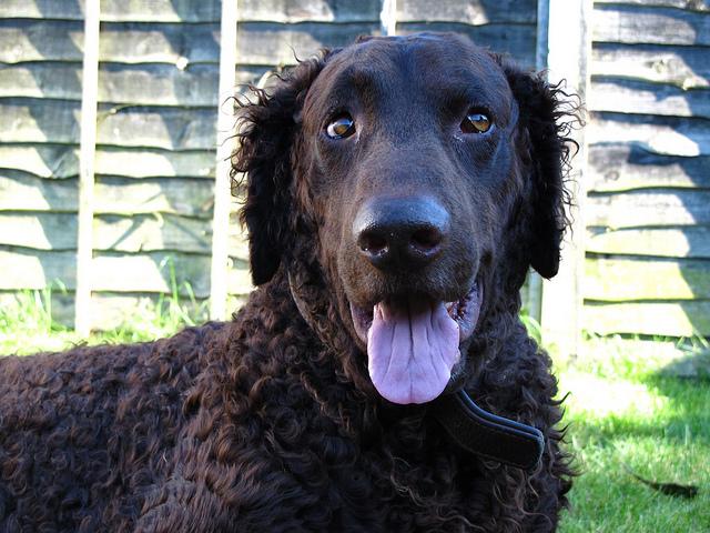
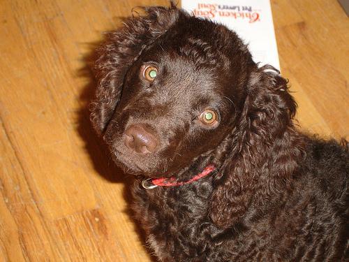
It is not difficult to find other dog breed pairs with minimal inter-class variation (for instance, Curly-Coated Retrievers and American Water Spaniels).
| Curly-Coated Retriever | American Water Spaniel |
|---|---|
 |
 |
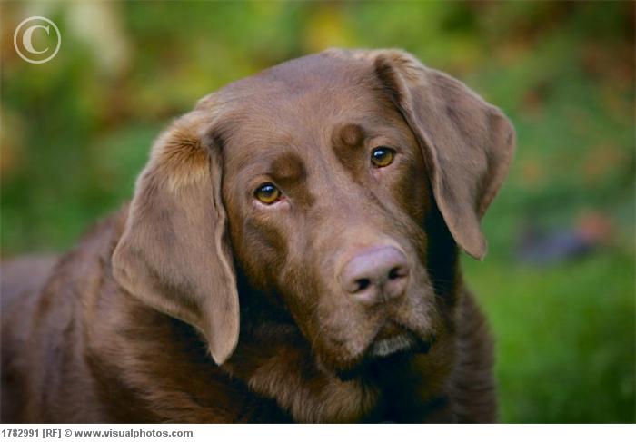
Likewise, recall that labradors come in yellow, chocolate, and black. Your vision-based algorithm will have to conquer this high intra-class variation to determine how to classify all of these different shades as the same breed.
| Yellow Labrador | Chocolate Labrador | Black Labrador |
|---|---|---|
 |
 |
 |
We also mention that random chance presents an exceptionally low bar: setting aside the fact that the classes are slightly imabalanced, a random guess will provide a correct answer roughly 1 in 133 times, which corresponds to an accuracy of less than 1%.
Remember that the practice is far ahead of the theory in deep learning. Experiment with many different architectures, and trust your intuition. And, of course, have fun!
Pre-process the Data
We rescale the images by dividing every pixel in every image by 255.
from PIL import ImageFile
ImageFile.LOAD_TRUNCATED_IMAGES = True

# pre-process the data for Keras
train_tensors = paths_to_tensor(train_files).astype('float32')/255
valid_tensors = paths_to_tensor(valid_files).astype('float32')/255
test_tensors = paths_to_tensor(test_files).astype('float32')/255
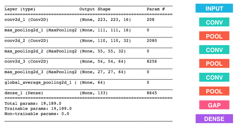
(IMPLEMENTATION) Model Architecture
Create a CNN to classify dog breed. At the end of your code cell block, summarize the layers of your model by executing the line:
model.summary()
We have imported some Python modules to get you started, but feel free to import as many modules as you need. If you end up getting stuck, here's a hint that specifies a model that trains relatively fast on CPU and attains >1% test accuracy in 5 epochs:
Question 4: Outline the steps you took to get to your final CNN architecture and your reasoning at each step. If you chose to use the hinted architecture above, describe why you think that CNN architecture should work well for the image classification task.
Answer:
I chose the architecture above, since I had not much hope on getting very good from scratch and wanted to rather spend my time on assessing the Transfer Learning with the given models.
Why does the given architecture work?
- The
input_shapeis given by the shape of the input tensors, which is(224, 224, 3). - The sequence convolutional layer - maxpooling layer multiple times is standard. The convolutional layer is filtering features (2 in this case) and the maxppoling layer is doing the abstraction.
padding=validworks here, since the borders are of no interest to us.- The activation functions 'relu' for the convolutional layers in the intermediate layers counteracts the disappearing gradient problem.
- Global Average pooling before the final layer helps to bring the complexity down before the dense layer and can also be interpreted as making a final abstraction
- Softmax is used in the Dense Layer, because this is a multiclass classification problem
Strides=2works since we are interested in the details and want things to be invariant against translations.
from keras.layers import Conv2D, MaxPooling2D, GlobalAveragePooling2D
from keras.layers import Dropout, Flatten, Dense
from keras.models import Sequential

model = Sequential()

### TODO: Define your architecture.
model.add(Conv2D(filters=16, kernel_size=2, strides=1, padding='valid',
    activation='relu', input_shape=(224, 224, 3)))
model.add(MaxPooling2D(pool_size=2, strides=2, padding='valid'))
model.add(Conv2D(filters=32, kernel_size=2, strides=1, padding='valid',
    activation='relu', input_shape=(111, 111, 16)))
model.add(MaxPooling2D(pool_size=2, strides=2, padding='valid'))
model.add(Conv2D(filters=64, kernel_size=2, strides=1, padding='valid',
    activation='relu', input_shape=(55, 55, 16)))
model.add(MaxPooling2D(pool_size=2, strides=2, padding='valid'))
model.add(GlobalAveragePooling2D())
model.add(Dense(133, activation='softmax'))

model.summary()
Compile the Model
model.compile(optimizer='rmsprop', loss='categorical_crossentropy', metrics=['accuracy'])
(IMPLEMENTATION) Train the Model
Train your model in the code cell below. Use model checkpointing to save the model that attains the best validation loss.
You are welcome to augment the training data, but this is not a requirement.
Run Option
I made another switch RECOMPUTE_BREED_DETECTOR_FROM_SCRATCH so that you can decide whether you want to run the module computation again or just use the computed weights from file.
RECOMPUTE_BREED_DETECTOR_FROM_SCRATCH = False
from keras.callbacks import ModelCheckpoint

if RECOMPUTE_BREED_DETECTOR_FROM_SCRATCH:
    ### TODO: specify the number of epochs that you would like to use to train the model.

    epochs = 5

    ### Do NOT modify the code below this line.

    checkpointer = ModelCheckpoint(filepath='saved_models/weights.best.from_scratch.hdf5',
                                   verbose=1, save_best_only=True)

    model.fit(train_tensors, train_targets,
              validation_data=(valid_tensors, valid_targets),
              epochs=epochs, batch_size=20, callbacks=[checkpointer], verbose=1)
else:
    print("""if run with RECOMPUTE_BREED_DETECTOR_FROM_SCRATCH, this cell produces the following output:
    Train on 6680 samples, validate on 835 samples
Epoch 1/5
6660/6680 [============================>.] - ETA: 0s - loss: 4.8823 - acc: 0.0093Epoch 00000: val_loss improved from inf to 4.86867, saving model to saved_models/weights.best.from_scratch.hdf5
6680/6680 [==============================] - 242s - loss: 4.8824 - acc: 0.0093 - val_loss: 4.8687 - val_acc: 0.0144
Epoch 2/5
6660/6680 [============================>.] - ETA: 0s - loss: 4.8594 - acc: 0.0132Epoch 00001: val_loss improved from 4.86867 to 4.84382, saving model to saved_models/weights.best.from_scratch.hdf5
6680/6680 [==============================] - 240s - loss: 4.8593 - acc: 0.0132 - val_loss: 4.8438 - val_acc: 0.0144
Epoch 3/5
6660/6680 [============================>.] - ETA: 0s - loss: 4.8145 - acc: 0.0168Epoch 00002: val_loss improved from 4.84382 to 4.80621, saving model to saved_models/weights.best.from_scratch.hdf5
6680/6680 [==============================] - 238s - loss: 4.8147 - acc: 0.0168 - val_loss: 4.8062 - val_acc: 0.0132
Epoch 4/5
6660/6680 [============================>.] - ETA: 0s - loss: 4.7723 - acc: 0.0197Epoch 00003: val_loss improved from 4.80621 to 4.78778, saving model to saved_models/weights.best.from_scratch.hdf5
6680/6680 [==============================] - 234s - loss: 4.7717 - acc: 0.0198 - val_loss: 4.7878 - val_acc: 0.0120
Epoch 5/5
6660/6680 [============================>.] - ETA: 0s - loss: 4.7391 - acc: 0.0207Epoch 00004: val_loss improved from 4.78778 to 4.76081, saving model to saved_models/weights.best.from_scratch.hdf5
6680/6680 [==============================] - 234s - loss: 4.7393 - acc: 0.0207 - val_loss: 4.7608 - val_acc: 0.0299
""")
Load the Model with the Best Validation Loss
model.load_weights('saved_models/weights.best.from_scratch.hdf5')
Test the Model
Try out your model on the test dataset of dog images. Ensure that your test accuracy is greater than 1%.
# get index of predicted dog breed for each image in test set
dog_breed_predictions = [np.argmax(model.predict(np.expand_dims(tensor, axis=0))) for tensor in test_tensors]

# report test accuracy
test_accuracy = 100*np.sum(np.array(dog_breed_predictions)==np.argmax(test_targets, axis=1))/len(dog_breed_predictions)
print('Test accuracy: %.4f%%' % test_accuracy)
bottleneck_features = np.load('bottleneck_features/DogVGG16Data.npz')
train_VGG16 = bottleneck_features['train']
valid_VGG16 = bottleneck_features['valid']
test_VGG16 = bottleneck_features['test']
Model Architecture
The model uses the the pre-trained VGG-16 model as a fixed feature extractor, where the last convolutional output of VGG-16 is fed as input to our model. We only add a global average pooling layer and a fully connected layer, where the latter contains one node for each dog category and is equipped with a softmax.
VGG16_model = Sequential()
VGG16_model.add(GlobalAveragePooling2D(input_shape=train_VGG16.shape[1:]))
VGG16_model.add(Dense(133, activation='softmax'))

VGG16_model.summary()
Compile the Model
VGG16_model.compile(loss='categorical_crossentropy', optimizer='rmsprop', metrics=['accuracy'])
Train the Model
checkpointer = ModelCheckpoint(filepath='saved_models/weights.best.VGG16.hdf5',
                               verbose=1, save_best_only=True)

VGG16_model.fit(train_VGG16, train_targets,
          validation_data=(valid_VGG16, valid_targets),
          epochs=20, batch_size=20, callbacks=[checkpointer], verbose=1)
Load the Model with the Best Validation Loss
VGG16_model.load_weights('saved_models/weights.best.VGG16.hdf5')
Test the Model
Now, we can use the CNN to test how well it identifies breed within our test dataset of dog images. We print the test accuracy below.
# get index of predicted dog breed for each image in test set
VGG16_predictions = [np.argmax(VGG16_model.predict(np.expand_dims(feature, axis=0))) for feature in test_VGG16]

# report test accuracy
test_accuracy = 100*np.sum(np.array(VGG16_predictions)==np.argmax(test_targets, axis=1))/len(VGG16_predictions)
print('Test accuracy: %.4f%%' % test_accuracy)
Predict Dog Breed with the Model
# from extract_bottleneck_features import *
Why I did not use the provided extract_bottleneck_features.py
It turned out to be a performance bottleneck, because:
- the model is reinitiated at every prediction
- the model initiation took about a second each time.
In my code below the models is defined only once: that makes the predictions a lot faster.
# My own version of extract bottleneck feature since the provided version was too slow:
from keras.applications.vgg16 import VGG16
from keras.applications.vgg16 import preprocess_input as vgg16_preprocess_input
from keras.applications.vgg19 import VGG19
from keras.applications.vgg19 import preprocess_input as vgg19_preprocess_input
from keras.applications.resnet50 import ResNet50
from keras.applications.resnet50 import preprocess_input as resnet50_preprocess_input
from keras.applications.xception import Xception
from keras.applications.xception import preprocess_input as xception_preprocess_input
from keras.applications.inception_v3 import InceptionV3
from keras.applications.inception_v3 import preprocess_input as inception_v3_preprocess_input

# initiating all models
model_imagenet_vgg16 = VGG16(weights='imagenet', include_top=False)
model_imagenet_vgg19 = VGG19(weights='imagenet', include_top=False)
model_imagenet_resnet50 = ResNet50(weights='imagenet', include_top=False)
model_imagenet_xception = Xception(weights='imagenet', include_top=False)
model_imagenet_inception_v3 = InceptionV3(weights='imagenet', include_top=False)


# extracting the bottleneck features from the models with the specific preprocessing ahead
def extract_VGG16(tensor):
    return model_imagenet_vgg16.predict(vgg16_preprocess_input(tensor))

def extract_VGG19(tensor):
    return model_imagenet_vgg19.predict(vgg19_preprocess_input(tensor))

def extract_Resnet50(tensor):
    return model_imagenet_resnet50.predict(resnet50_preprocess_input(tensor))

def extract_Xception(tensor):
    return model_imagenet_xception.predict(xception_preprocess_input(tensor))

def extract_InceptionV3(tensor):
    return model_imagenet_inception_v3.predict(inception_v3_preprocess_input(tensor))
def VGG16_predict_breed(img_path):
    # extract bottleneck features
    bottleneck_feature = extract_VGG16(path_to_tensor(img_path))
    # obtain predicted vector
    predicted_vector = VGG16_model.predict(bottleneck_feature)
    # return dog breed that is predicted by the model
    return dog_names[np.argmax(predicted_vector)]
Testing the VGG Breed Detector on the Dog Files
# getting the breed from the path name as ground truth
def get_breed(img_path):
    path_components = img_path.split('/')
    breed_component = path_components[2]
    breed = breed_component.split('.')[1]
    return breed
# Calling my accuracy detector with the breed detector and the ground truth
get_detector_accurancy(title="Dog Breeds by VGG16",
                       img_path_list=dog_files_short,
                       detector=VGG16_predict_breed,
                       ground_truth=[get_breed(img_path) for img_path in dog_files_short],
                       show_fails=False)
Step 5: Create a CNN to Classify Dog Breeds (using Transfer Learning)
You will now use transfer learning to create a CNN that can identify dog breed from images. Your CNN must attain at least 60% accuracy on the test set.
In Step 4, we used transfer learning to create a CNN using VGG-16 bottleneck features. In this section, you must use the bottleneck features from a different pre-trained model. To make things easier for you, we have pre-computed the features for all of the networks that are currently available in Keras:
- VGG-19 bottleneck features
- ResNet-50 bottleneck features
- Inception bottleneck features
- Xception bottleneck features
The files are encoded as such:
Dog{network}Data.npz
where {network}, in the above filename, can be one of VGG19, Resnet50, InceptionV3, or Xception. Pick one of the above architectures, download the corresponding bottleneck features, and store the downloaded file in the bottleneck_features/ folder in the repository.
(IMPLEMENTATION) Obtain Bottleneck Features
In the code block below, extract the bottleneck features corresponding to the train, test, and validation sets by running the following:
bottleneck_features = np.load('bottleneck_features/Dog{network}Data.npz')
train_{network} = bottleneck_features['train']
valid_{network} = bottleneck_features['valid']
test_{network} = bottleneck_features['test']### TODO: Obtain bottleneck features from another pre-trained CNN.
My approach
In my opinion the features are very important for arriving at a good machine learning model. Therefore I decided to vizualize and compare all suggested bottleneck features with TSNE, before deciding upon which dataset I want to install my transfer learning.
Step 1 Getting bottleneck features for all networks
Getting Training Bottleneck features
In order to compare the networks I used the features for the training datasets. I needed the training data for this since with 133 classes and 6680 this is about 50 dogs per breed in average. This is enough to get an idea, whether dogs of the same breed are close regarding their features. The validation data with just about 800 dogs would not have given meaningful results in that regard.
Xception Bottleneck Features
I could not open the provided bottleneck dataset for the Xception features. It gave me an error 'bad file' or something similar, when I tried to load it. I therefore recalculated the features and stored them in my own file locally. The file is not on github, since it was to big to store it there.
Run Options
Since computing the TSNE projection is time expensive, I stored the TSNE projection images in a file and give the option to recompute them with the variable RECOMPUTE_TSNE_PROJECTIONS, which is preset to False, but can be changed to True.
RECOMPUTE_TSNE_PROJECTIONS = True
# Networks
RESNET50 = 'ResNet50'
VGG19 = 'VGG19'
INCEPTIONV3 = 'InceptionV3'
XCEPTION = 'Xception'
networks = [VGG19, RESNET50, INCEPTIONV3, XCEPTION]
if RECOMPUTE_TSNE_PROJECTIONS:
    # Get bottleneck features
    train_features = {}

    # Bottleneck features for ResNet50: training data for comparing the networks
    bottleneck_features_resnet50 = np.load('bottleneck_features/DogResnet50Data.npz')
    train_features[RESNET50] = bottleneck_features_resnet50['train']

    # Bottleneck features for VGG19: training data for comparing the networks
    bottleneck_features_vgg19 = np.load('bottleneck_features/DogVGG19Data.npz')
    train_features[VGG19] = bottleneck_features_vgg19['train']

    # Bottleneck features for InceptionV3: training data for comparing the networks
    bottleneck_features_inceptionv3 = np.load('bottleneck_features/DogInceptionV3Data.npz')
    train_features[INCEPTIONV3] = bottleneck_features_inceptionv3['train']

    # Xception Bottleneck features for train data: see above for the reasons why I compute them myself
    try:
        train_features[XCEPTION] = np.load('myfiles/bottleneckfeatures/DogXceptionDataTrain.npy')
    except FileNotFoundError:
        # initialize array
        train_features[XCEPTION] = np.zeros((tensors.shape[0],7,7,2048))
        # compute features from pretrained Xception network
        for i in tqdm(range(tensors.shape[0])):
            train_features[XCEPTION][i] = extract_Xception(np.expand_dims(tensors[i], axis=0))
        # saving the bottleneckfeatures for later
        np.save('myfiles/bottleneckfeatures/DogXceptionDataTrain', train_features[XCEPTION])
    else:
        print("Loaded {} Xception features from file".format(len(train_features[XCEPTION])))

    # print out the result
    for network in networks:
        print("bottleneck features of {} have shape {}".format(network, train_features[network].shape))
else:
    print("""if run with RECOMPUTE_TSNE_PROJECTIONS, this cell produces the following output:
    Loaded 6680 Xception features from file
    bottleneck features of VGG19 have shape (6680, 7, 7, 512)
    bottleneck features of ResNet50 have shape (6680, 1, 1, 2048)
    bottleneck features of InceptionV3 have shape (6680, 5, 5, 2048)
    bottleneck features of Xception have shape (6680, 7, 7, 2048)""")
(IMPLEMENTATION) Model Architecture
Create a CNN to classify dog breed. At the end of your code cell block, summarize the layers of your model by executing the line:
<your model's name>.summary()
Question 5: Outline the steps you took to get to your final CNN architecture and your reasoning at each step. Describe why you think the architecture is suitable for the current problem.
Answer:
if RECOMPUTE_TSNE_PROJECTIONS:
    # reshape features to one dimension
    train_features_2d = {}

    for network in networks:
        m, h, h, n = train_features[network].shape
        train_features_2d[network] = train_features[network].reshape(m, h*h*n)
        print("Features of {} have now shape {}".format(network, train_features_2d[network].shape))
else:
    print("""if run with RECOMPUTE_TSNE_PROJECTIONS, this cell produces the following output:
    Features of VGG19 have now shape (6680, 25088)
    Features of ResNet50 have now shape (6680, 2048)
    Features of InceptionV3 have now shape (6680, 51200)
    Features of Xception have now shape (6680, 100352)""")
if RECOMPUTE_TSNE_PROJECTIONS:
    tsne_proj = {}
    for network in networks:
        filename = "Dog" + network + "TrainTSNE.npy"
        filepath = '/'.join(['myfiles', 'tsnedata', filename])
        try:
            tsne_proj[network] = np.load(filepath)
        except FileNotFoundError:
            # initialize array
            tsne_proj[network] = perform_tsne(train_features_2d[network])
            # saving the bottleneckfeatures for later
            np.save(filepath, tsne_proj[network] )
            print("Computed TSNE projection for network {} and save it to file {}".format(network, filepath))
        else:
            print("Loaded TSNE projection for network {} from file {}".format(network, filepath))
else:
    print("""if run with RECOMPUTE_TSNE_PROJECTIONS, this cell produces the following output:
    Loaded TSNE projection for network VGG19 from file myfiles/tsneprojectionsData/DogVGG19TrainTSNE.npy
    Loaded TSNE projection for network ResNet50 from file myfiles/tsneprojectionsData/DogResNet50TrainTSNE.npy
    Loaded TSNE projection for network InceptionV3 from file myfiles/tsneprojectionsData/DogInceptionV3TrainTSNE.npy
    Loaded TSNE projection for network Xception from file myfiles/tsneprojectionsData/DogXceptionTrainTSNE.npy""")
Step 3 Helper functions for plotting the projections
Helper Functions for breed encodings
I programed some helper functions to get from target (one hot coded) to code and breed names
Helper Functions for coloring of the map and building the legend
I decided to show only a number of breeds and have an other color for breeds that have not been selected for visualization.
# helper functions
DOGFILEPATTERN = "dogImages/train/*/"

# load list of dog names
dog_codes = [item[16:-1].split('.') for item in sorted(glob(DOGFILEPATTERN))]
dog_codes = {int(c[0]): c[1] for c in dog_codes}

# get breed name from one hot encoding
def get_breed_from_target(target):
    return dog_codes[get_code_from_target]

# get breed code from one hot encoding
def get_code_from_target(target):
    return np.argmax(target) + 1

# get breed name from breed code
def get_breed_from_code(code):
    return dog_codes[code]

# get breed code from breed name
def get_code_from_breed(name):
    return [c for c, n in dog_codes.items() if n == name][0]
# prepare the tsne coloring and legend
# Parameters:
# - selected_breed_codes: small number of codes of breeds, that have been selected for visualization
# - train_targets: targets in one hot encoding
# Returns
# - legend with breed names and color codes, including a code for 'other_breeds'
# - target in color codes: non selected breeds get the code for the 'other breeds' color.
def get_coloring_for_breeds(selected_breed_codes, train_targets):
    # count selected breeds
    selected_breed_count = len(selected_breed_codes)
    # get selected breed names
    selected_breed_names = [get_breed_from_code(code) for code in selected_breed_codes]

    # build legend
    legend = {i: selected_breed_names[i] for i in range(selected_breed_count)}
    # the last entry is 'other breeds'
    legend[selected_breed_count] = 'other breeds'

    # build color map for selected breeds: breed code -> position in the selection of breed codes
    # that way the colors are defined as a range sequence 0,1,2,3, ..., selected_breed_count-1
    color_map = {}
    for code in selected_breed_codes:
        color_map[code] = selected_breed_codes.index(code)

    # transform 1 hot encoding into breed codes
    train_target_codes = np.apply_along_axis(get_code_from_target, 1, train_targets)
    # transform breed codes into color codes
    colors = np.full((train_targets.shape[0]), selected_breed_count)
    for i in range(len(colors)):
        if train_target_codes[i] in color_map:
            colors[i] = color_map[train_target_codes[i]]

    # return legend and the target transformed into color codes
    return colors, legend
Step 4 Plotting the projections
- I do this network by network since the plot for a network is already big enough.
- since I use seaborn for this which was not part of the installed libraries for this project: the plots are fetched from file in the case that seaborn is not installed
if RECOMPUTE_TSNE_PROJECTIONS:
    # get random breed codes
    random_breed_codes = [random.randint(1, 133) for r in range(9)]
    # build legend and colors for them
    colors, legend = get_coloring_for_breeds(random_breed_codes, train_targets)
# visualize TSNE
# Now we call the scatter plot function on our data

# plot TSNE projection

file_path = 'myfiles/tsneplots/DogBreedsVGG19TSNE.png'
if RECOMPUTE_TSNE_PROJECTIONS:
    network = 'VGG19'
    scatter(tsne_proj[network],
            colors,
            legend,
            title="Dog Features for {}".format(network),
            file_path=file_path,
            other_color=True)
else:
    show_image_original(file_path)

# Resnet50
file_path = 'myfiles/tsneplots/DogBreedsResnet50TSNE.png'
if RECOMPUTE_TSNE_PROJECTIONS:
    network = 'ResNet50'
    scatter(tsne_proj[network],
            colors,
            legend,
            title="Dog Features for {}".format(network),
            file_path=file_path,
            other_color=True)
else:
    show_image_original(file_path)

# InceptionV3
file_path = 'myfiles/tsneplots/DogBreedsInceptionV3TSNE.png'
if RECOMPUTE_TSNE_PROJECTIONS:
    network = 'InceptionV3'
    scatter(tsne_proj[network],
            colors,
            legend,
            title="Dog Features for {}".format(network),
            file_path=file_path,
            other_color=True)
else:
    show_image_original(file_path)

# Xception
file_path = 'myfiles/tsneplots/DogBreedsXceptionTSNE.png'
if RECOMPUTE_TSNE_PROJECTIONS:
    network = 'Xception'
    scatter(tsne_proj[network],
            colors,
            legend,
            title="Dog Features for {}".format(network),
            file_path=file_path,
            other_color=True)
else:
    show_image_original(file_path)

Result
- ResNet50, Xception and InceptionV3 all look good.
Decision: I choose
- InceptionV3
- ResNet50
Both look good and my idea is to combine their preditions in order to be able to detect dogs that are not pure breeds better.
InceptionV3 Model
### Define your architecture.

# Shape of InceptionV3:
print("InceptionV3 bottleneck features are of shape {}.".format(train_features['InceptionV3'].shape[1:]))
# getting the train, test and validation features for InceptionV3
bottleneck_features_inceptionv3 = np.load('bottleneck_features/DogInceptionV3Data.npz')
train_InceptionV3 = bottleneck_features_inceptionv3['train']
valid_InceptionV3 = bottleneck_features_inceptionv3['valid']
test_InceptionV3 = bottleneck_features_inceptionv3['test']
# I decide to squeeze the input shapes:
print("Shape of the Input for InceptionV3 is ", train_InceptionV3.shape[1:])
Define the Transfer Learning Model
# Architecture is simple since the features are already very good
InceptionV3_model = Sequential()
InceptionV3_model.add(GlobalAveragePooling2D(input_shape=train_InceptionV3.shape[1:]))
InceptionV3_model.add(Dense(133, activation='softmax'))

InceptionV3_model.summary()
Compile the Model
### TODO: Compile the model.
InceptionV3_model.compile(loss='categorical_crossentropy', optimizer='adam', metrics=['accuracy'])
Train the Model
### TODO: Train the model.
checkpointer = ModelCheckpoint(filepath='saved_models/weights.best.InceptionV3.hdf5',
                               verbose=1, save_best_only=True)

InceptionV3_model.fit(train_InceptionV3, train_targets,
          validation_data=(valid_InceptionV3, valid_targets),
          epochs=10, batch_size=100, callbacks=[checkpointer], verbose=1)
Load the Model with the Best Validation Loss
### TODO: Load the model weights with the best validation loss.
InceptionV3_model.load_weights('saved_models/weights.best.InceptionV3.hdf5')
Test the Model
Try out your model on the test dataset of dog images. Ensure that your test accuracy is greater than 60%.
### TODO: Calculate classification accuracy on the test dataset.
# get index of predicted dog breed for each image in test set
InceptionV3_predictions = [np.argmax(InceptionV3_model.predict(np.expand_dims(feature, axis=0)))
                           for feature in test_InceptionV3]

# report test accuracy
test_accuracy = 100*np.sum(np.array(InceptionV3_predictions)==np.argmax(test_targets, axis=1))/len(InceptionV3_predictions)
print('Test accuracy: %.4f%%' % test_accuracy)
ResNet50 Model
# getting the train, test and validation features for ResNet50
bottleneck_features_resnet50 = np.load('bottleneck_features/DogResNet50Data.npz')
train_ResNet50 = bottleneck_features_resnet50['train']
valid_ResNet50 = bottleneck_features_resnet50['valid']
test_ResNet50 = bottleneck_features_resnet50['test']
# I decide to squeeze the input shapes:
train_ResNet50 = np.squeeze(train_ResNet50)
valid_ResNet50 = np.squeeze(valid_ResNet50)
test_ResNet50 = np.squeeze(test_ResNet50)
#### define the model
ResNet50_TL_model = Sequential()
ResNet50_TL_model.add(Dense(133, input_shape=train_ResNet50.shape[1:], activation='softmax'))
ResNet50_TL_model.summary()
Compile the model
ResNet50_TL_model.compile(loss='categorical_crossentropy', optimizer='adam', metrics=['accuracy'])
Train the model
### TODO: Train the model.
checkpointer = ModelCheckpoint(filepath='saved_models/weights.best.ResNet50_TL_model.hdf5',
                               verbose=1, save_best_only=True)

ResNet50_TL_model.fit(train_ResNet50, train_targets,
          validation_data=(valid_ResNet50, valid_targets),
          epochs=10, batch_size=20, callbacks=[checkpointer], verbose=1)
### TODO: Load the model weights with the best validation loss.
ResNet50_TL_model.load_weights('saved_models/weights.best.ResNet50_TL_model.hdf5')
### TODO: Calculate classification accuracy on the test dataset.
# get index of predicted dog breed for each image in test set
ResNet50_TL_predictions = [np.argmax(ResNet50_TL_model.predict(np.expand_dims(feature, axis=0)))
                        for feature in test_ResNet50]

# report test accuracy
test_accuracy = 100*np.sum(np.array(ResNet50_TL_predictions)==np.argmax(test_targets, axis=1))/len(ResNet50_TL_predictions)
print('Test accuracy: %.4f%%' % test_accuracy)
Compare the two models
m_test = len(test_targets)
m_diff = len([i for i in range(m_test) if InceptionV3_predictions[i]!=ResNet50_TL_predictions[i]])
print("The two models don't agree in {} % of the cases".format(round(m_diff / m_test * 100, 2)))
Combine the two models
I am just combining the predictions here:
- both models give a prediction for the breed
- I choose the prediction of the model that has the higher probability on its prediction
# helper function that combines the prediction of the two models
def combined_prediction(ResNet50_feature, InceptionV3_feature):
    resnet50_pred = ResNet50_TL_model.predict(np.expand_dims(ResNet50_feature, axis=0))
    inceptionv3_pred = InceptionV3_model.predict(np.expand_dims(InceptionV3_feature, axis=0))
    if resnet50_pred[0, np.argmax(resnet50_pred)] > inceptionv3_pred[0, np.argmax(inceptionv3_pred)]:
        return np.argmax(resnet50_pred)
    else:
        return np.argmax(inceptionv3_pred)

# getting the combined predictions for the test data
combined_predictions = [combined_prediction(test_ResNet50[i], test_InceptionV3[i]) for i in range(len(test_ResNet50))]
# computing the accuracy of the combined predictions on the test data
test_accuracy = 100*np.sum(np.array(combined_predictions)==np.argmax(test_targets, axis=1))/len(ResNet50_TL_predictions)
print('Test accuracy: %.4f%%' % test_accuracy)
(IMPLEMENTATION) Predict Dog Breed with the Model
Write a function that takes an image path as input and returns the dog breed (Affenpinscher, Afghan_hound, etc) that is predicted by your model.
Similar to the analogous function in Step 5, your function should have three steps:
- Extract the bottleneck features corresponding to the chosen CNN model.
- Supply the bottleneck features as input to the model to return the predicted vector. Note that the argmax of this prediction vector gives the index of the predicted dog breed.
- Use the
dog_namesarray defined in Step 0 of this notebook to return the corresponding breed.
The functions to extract the bottleneck features can be found in extract_bottleneck_features.py, and they have been imported in an earlier code cell. To obtain the bottleneck features corresponding to your chosen CNN architecture, you need to use the function
extract_{network}
where {network}, in the above filename, should be one of VGG19, Resnet50, InceptionV3, or Xception.
### TODO: Write a function that takes a path to an image as input
### and returns the dog breed that is predicted by the model.
def combined_models_predict_breed(img_path):
    inceptionv3_feature = np.squeeze(extract_InceptionV3(path_to_tensor(img_path)))
    resnet50_feature = np.squeeze(extract_Resnet50(path_to_tensor(img_path)))
    # reshape the features
    prediction = combined_prediction(resnet50_feature, inceptionv3_feature)
    breed = dog_names[prediction]
    return breed
I am doing this for the combined prediction of both models above
# Calling my accuracy detector with the breed detector and the ground truth
get_detector_accurancy(title="Dog Breeds by Combined InceptionV3 and ResNet50 Transfer Learning Model",
                       img_path_list=dog_files_short,
                       detector=combined_models_predict_breed,
                       ground_truth=[get_breed(img_path) for img_path in dog_files_short],
                       show_fails=True)
Step 6: Write your Algorithm
Write an algorithm that accepts a file path to an image and first determines whether the image contains a human, dog, or neither. Then,
- if a dog is detected in the image, return the predicted breed.
- if a human is detected in the image, return the resembling dog breed.
- if neither is detected in the image, provide output that indicates an error.
You are welcome to write your own functions for detecting humans and dogs in images, but feel free to use the face_detector and dog_detector functions developed above. You are required to use your CNN from Step 5 to predict dog breed.
Some sample output for our algorithm is provided below, but feel free to design your own user experience!
(IMPLEMENTATION) Write your Algorithm
What I am using
- my
dog_human_many_other_detectorfrom above to decide whether the image is valid - my breed detector for the breed
### TODO: Write your algorithm.
### Feel free to use as many code cells as needed.
import matplotlib.image as mpimg

def format_breed(breed):
    words = breed.split('_')
    words = [word.capitalize() for word in words]
    return ' '.join(words)

def process_img(img_path):
    show_image(img_path)
    try:
        species = DogHumanOtherDetector(img_path)
    except ValueError as e:
        print("Error: {}. Please show me another picture!".format(e))
    else:
        breed = combined_models_predict_breed(img_path)
        print("Hello {},".format(species.name))
        if species == Species.HUMAN:
            print("your are most similar to the dog breeds {}".format(format_breed(breed)))
        else:
            print("I recognize your breed! You are a {}.".format(format_breed(breed)))
Step 7: Test Your Algorithm
In this section, you will take your new algorithm for a spin! What kind of dog does the algorithm think that you look like? If you have a dog, does it predict your dog's breed accurately? If you have a cat, does it mistakenly think that your cat is a dog?
(IMPLEMENTATION) Test Your Algorithm on Sample Images!
Test your algorithm at least six images on your computer. Feel free to use any images you like. Use at least two human and two dog images.
Question 6: Is the output better than you expected :) ? Or worse :( ? Provide at least three possible points of improvement for your algorithm.
Answer:
## TODO: Execute your algorithm from Step 6 on
## at least 6 images on your computer.
## Feel free to use as many code cells as needed.
# a cat
process_img('myfiles/testimages/cat.jpg')

# a computer
process_img('myfiles/testimages/computerdesk.jpg')

# a parrot
process_img('myfiles/testimages/parrot.jpg')

# family with a dog
process_img('myfiles/testimages/obama-family.jpg')

# a pure breed labrador
process_img('myfiles/testimages/labradorwelpe.jpg')

# a mixed breed
process_img('myfiles/testimages/mixed_dog.jpg')

# two dogs: one big, one small
process_img('myfiles/testimages/2dogs.jpg')

# a woman
process_img('myfiles/testimages/woman_greyhaired.jpg')

# a mixed breed "cookapoo"
process_img('myfiles/testimages/cookapoo.jpg')

# a couple of different breeds
process_img('myfiles/testimages/severaldogs.jpg')

# a woman in profile
process_img('myfiles/testimages/young-woman-profile.jpg')

Is the output better than you expected :) ? Or worse :( ?
I am quite happy with the output of my algorithm now. But it took me a while to get there.
Provide at least three possible points of improvement for your algorithm.
- In order to detect multiple dogs or humans, data labled with the number of dogs and humans could help.
- Without new data, I could also try to exploit the probabilities returned by the breed detecting models further: they can help to detect multiple breeds, if the prediction of several breeds are above a threshold. That could indicate mixed breeds or more then one dog of different breeds.
- The two dog breed detecting models could be combined in other ways: by taking the mean of all predictions for example. I could also combine even more models, such as adding a model derived from Xception bottleneck features to the mix.
What I learned:
- The most important thing that I learned in this practice is that the algorithm will just learn what you train them for.
In this case we had just data for humans and dogs and wanted the algorithm to detect if it was not a human or thing. This was only possible by using the Imagenet Classifier for ResNet50 above, since it was trained on a whole range of images and could pick out dogs from everything else.
- Combining algorithms helps to get better results
Even though both bottleneck features I tried gave good result, their combined result was even better
- Getting to Apps from models can be achieved by combining classifiers with a different focus
The App would not have been possible to derive from a single Classifier without a huge amount of additinal data, but by combining several algorithms in a smart way, it was possible to build the app and make it reject images that were neither human or dog even though it was never trained on such images. This was acchieved by using a ready made Classifier from Keras, that had not much to do with the task at hand.
- Transfer Learning is very powerful!
Distinguishing the dog breeds is quite hard. I could never do this with 86% accuracy. So I am impressed how easy it was to build such a powerful classfier with transfer learning.